Tim Dunbar

Benford’s Law Explained

Benford’s law is also called the first digit law, it’s an observation about the frequency distribution of the most significant digits in any series of numbers. It turns out that roughly 30% of the numbers should start with the number 1, roughly 20% of the numbers should start with 2, and so on. Benford’s law is usually used as a kind of “canary” for fraud. In other words if the set of numbers in the dataset do not conform to Benford’s law there might be some manipulation going on and further investigation is required.

This is just a quick rundown of the probablility formula for Benford’s law. So for leading digit d such that

\[ d\in{1, 2, …, 9} \]

The formulas is…

Because the log of the quotient is the difference of the logs and vice versa we can…

And finally…

Now on with the fun stuff

Administrative stuff, package loading, variables, etc.

As always we need to load the libraries we are going to use as well as the data into a dataframe.

library(readr)
library(dplyr)
library(ggplot2)
ghent_df<-readr::read_csv("~/Naggle/GhentDataSetTrain.csv")

We need to filter out some stuff to prepare for Benford’s Law

There is at least one type of construction represented in this dataset that needs to be filtered out (there might be more in fact). “Residential Outbuildings” seem to be listed seperately but they repeat the same values as the main residential structure they are attached with. Leaving this in will make the analysis less accurate.

filtered_ghent_df<-dplyr::filter(ghent_df, ghent_df$`Property Use`!="Residential Outbuilding")

Peel off the columns we are interested in (namely 2016 Land and 2016 Building)

In this analysis I’m only interested in two of the columns and really only the individual sums of those two columns. I want to use the total price of the properties in my analysis so I split out the assessed land value and the assessed building value and sum them.

benford_prep_df<-filtered_ghent_df[,c(11, 12)]

benford_prep_df<-dplyr::mutate(benford_prep_df, 'total' = benford_prep_df$`2016 Land`+benford_prep_df$`2016 Building`)

benford_prep_df<-dplyr::mutate(benford_prep_df, 'first_digit' = substr(benford_prep_df$total, 1, 1))

Peel off the first_digit column so that we can see how it conforms to Benford’s law

And now to simply count all the 1s, 2s, 3s, and so on using the table function in R.

benford_counts_firsts <- as.data.frame(benford_prep_df$first_digit)

benford_counts_table_firsts <- as.data.frame(table(benford_counts_firsts))
benford_counts_table_firsts <- dplyr::mutate(benford_counts_table_firsts, percentage = benford_counts_table_firsts$Freq/1737)

Firsts table

We cna already see that there is something interesting happening with 3s and 4s, and there doesn’t seem to be enough 1s.

head(benford_counts_table_firsts, 9)

##   benford_counts_firsts Freq percentage
## 1                     1  373 0.21473805
## 2                     2  293 0.16868164
## 3                     3  431 0.24812896
## 4                     4  270 0.15544041
## 5                     5  157 0.09038572
## 6                     6   82 0.04720783
## 7                     7   50 0.02878526
## 8                     8   51 0.02936097
## 9                     9   30 0.01727116

Histogram of the resulting counts for firsts

ggplot(benford_counts_firsts, aes(benford_counts_firsts$`benford_prep_df$first_digit`)) +
stat_count(binwidth=1, colour="black", fill="white") +
xlab("First Digit Counts") +
ylab("Counts") +
ggtitle("Benford's Law Analysis of Ghent Housing Data")

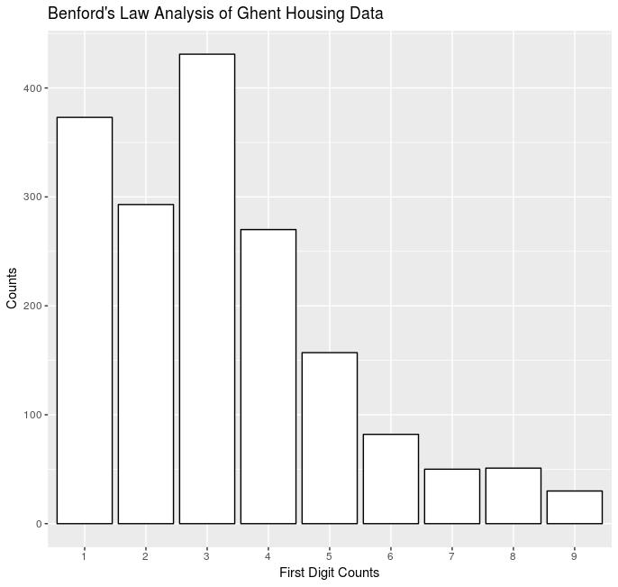
Conclusion

This data set does not comply with Benford’s law because more total assessed values begin with the number 3 then anything else and there are more 4s then there should be as well. This is not to say that there is fraud happening here but there is something interesting that would require further investigation beyond the scope of this post. However, most likely this is because Ghent is a mildly affluent neighborhood with a lot of expensive homes for the upper middle class folks.