Tim Dunbar

Moran’s I Explanation

Moran’s I is a measurement of how spatial information might correlate with some other variable. In this case I am comparing the Euclidean distance (from each other) of homes in the Ghent neighborhodd of Norfolk and their property values. I didn’t do a lot of cleaning of the data, preferring instead to get a baseline and to see how much the p value improved after cleaning.

As always we need our libraries

library(ggplot2)
library(dplyr)
library(RDSTK)
library(leaflet)
library(ape)
library(readr)

Here I am pulling out the columns I am interested in, specifically the complete address

df<-read_csv("~/Naggle/2017-07_GhentHousingData/data/GhentDataSetWithGeo.csv")

columns<-c(3, 5, 7, 8, 9, 10, 16, 17)

new_df<-df[,columns]

new_df$whole_address<-paste(new_df$`Property Street`, new_df$`Property City`, new_df$`Property State`, new_df$`Property Zip`)
new_df$total<-df$`2016 Building`+df$`2016 Land`

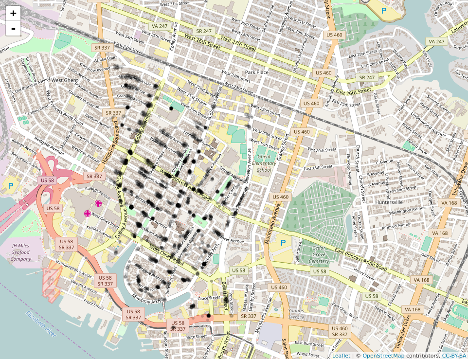
Let’s make a map so that we can perhaps get a sense of any clustering effects with the home values. One the below map, the darker the blue the higher the total property value of the address.

pal <- colorQuantile(c("blue"), domain = as.numeric(new_df$total))

leaflet() %>%
  addTiles() %>%
  addCircleMarkers(lng=new_df$longitude, lat=new_df$latitude, weight=3, radius=3, opacity=.2, color=pal)

Finally I calculate the Moran’s I of this dataset. the below p value of 0.375 is not as high as I thought it should be. It makes sense that like value homes will be close to each other, I mean it’s not often that one sees a mansion next to a trailer park. I will clean up the data and see if it can be improved.

xy<-new_df[,c(2,3,10)]

xy.dist<-as.matrix(dist(cbind(xy$longitude, xy$latitude), method = "euclidean", diag = FALSE, upper = FALSE, p = 2))

xy.dist.inv <-1/xy.dist

diag(xy.dist.inv)<-0
xy.dist.inv[xy.dist.inv == Inf] <- 0

Moran.I(xy$total, xy.dist.inv)

As seen below the p value is higher then .05 so the null hypothesis is not confirmed. There is a spatial correlation with property value.

$observed
[1] 0.001799266

$expected
[1] -0.0004823927

$sd
[1] 0.002575867

$p.value
[1] 0.3757347